What is Information Extraction from Receipts
Information extraction (IE) is the task of automatically extracting structured information from unstructured and/or semi-structured machine-readable documents.
For example, suppose your bank has created a phone app that allows you to schedule bill payments just by taking a picture of the bill, that could be divided in two steps: (1) recognize all the words in the picture and (2) look through the words until all the essential pieces of information have been identified, in particular, the amount due, the due date, and who to pay.
The first step is called Optical Character Recognition (OCR) and the second step is usually called Tagging, the essential part of Information Extraction.
Information Extraction from Receipts is special, because the Receipts, as well as other types of visually-rich documents (VRD), encode semantic information in their visual layout, so the Tagging step should not be done based solely on the machine readable words, but we should also inform it with the layout information or position of the word relative to the other words in the document.
An example of semantic information encoded in the layout would as follows: if a number is found immediately to the right of the words “Total Due:”, then this number must be the total due, with high probability; although this case looks deterministic enough to be tackled with a simple rule, other cases of information conveyed by the layout are not so obvious, like the list of products or services billed, which are usually presented in a table with column titles.
Optical Character Recognition (OCR)
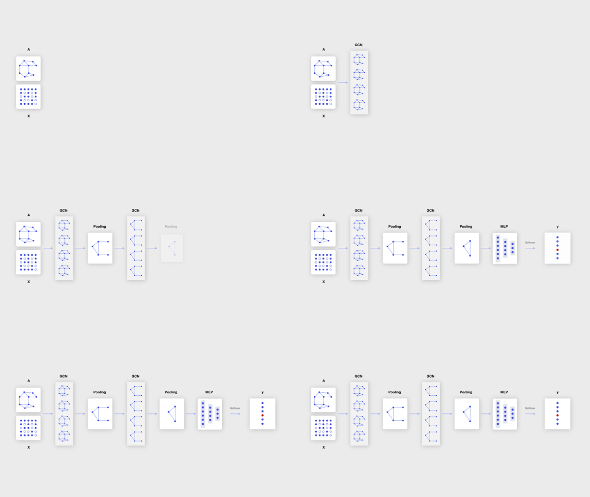
OCR deals with extracting characters or words from an image. The output needs to be extremely detailed and precise, capturing each character found on a page of text, for instance. Besides finding the coordinates of each character, OCR needs to figure out all manner of spatial details, like baselining, spacing, variations in fonts, for instance [1]:

More recently, a variety of deep learning-based text-extractors are been developed, allowing to tackle even more variability in the input, like noisy backgrounds [2] and hand-written characters [3].
Information Extraction (IE)
As we have seen before, the Information Extraction step consists mainly of classifying words (tagging), the output can be stored as key-value pairs in a computer-friendly file format (e.g.: JSON). The data extracted can then be efficiently archived, indexed and used for analytics.
If we compare OCR to young children training themselves to recognize characters and words, then Information Extraction would be like children learning to make sense of the words.
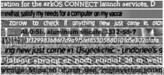
An example of IE would be when you stare at your credit card bill trying to find the amount due and the due date. Suppose you want to build an AI application to do it automatically; OCR could be applied to extract the text from the image, converting pixels into bytes or Unicode characters, and the output would be every single character printed in the bill.
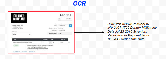
In order to use the output from OCR, first we need to apply an information extraction step to filter out all the irrelevant words and give you only the two items that you need: the date and the amount. In order to do that, IE needs to classify every word or character with a tag, for instance: “this is a dollar amount:, “this is a date”, “this is an address”, or “this is undefined”.
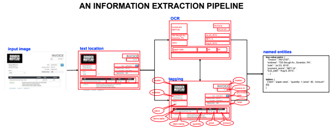
The following picture shows an Receipt IE pipeline, in which each text area of interest found by OCR is tagged with label indicating what class of information it contains, for instance “Amount Due”, “Address” or “Date”.
Traditional Approaches
There have been a number of efforts to perform the tagging process applying traditional techniques [4], most of them can be grouped into two large categories: template-based and NLP-based.
Template-Based
This approach starts by extracting the layout information, either by matching it to a known receipt format or by applying some rules to conclude what is the type of information contained in each position on the image.
For example, a system may be pre-configured with a set of known receipt formats and when a new receipt is scanned, it will try to classify the input image into one of the known layouts by matching keywords and using assumptions about the spatial layout and content of the fields.
The obvious drawback of this approach is that it cannot understand a receipt unless it matches one of the layouts previously known to the system.
Natural Language Processing (NLP)-based
This approach starts by converting the image into a text blob using OCR and then applies an NLP analysis technique known as Named Entity Recognition (NER) with the goal of assigning tags to each portion of the text. A tag is the equivalent of a field name in the image, it just indicates the type of information represented by the text, for example: “date” or “address”.
This approach is able to process new unseen layouts, but it breaks down with multiline text, like addresses and tables, where the information is embedded in the spatial arrangement of the layout, not in the text itself.
To address the limitations of the two approaches described above, a third approach to the tagging problem has been developed, this is called Graph Convolutional Networks (GCN).
Graph Convolutional Networks
The invention of GCNs is motivated by the following reasons [4]:
- The need to recognize local patterns in graphs, similarly to the way a CNN scans the input data through a small window recognizing local relations between the nodes within the window, a GCN could start by capturing local patterns between neighboring nodes in a graph (e.g.: the visual layout is a pattern that relates several adjacent text areas in a part of the image, like a table in an invoice).
- The need to recognize hierarchies of patterns. A CNN allows stacking many layers where the patterns recognized by the first layer are used as input to the second, which then learns to recognize combinations of patterns (e.g.: in an invoice, the table is usually below, the invoice number and above the total amount due
- Convolutions learn to recognize local patterns independently of variations in size or position in the input (translation invariance), provided that the training data contains such variability.
- Graphs are locally connected structures, which makes them a good candidate for the type of analysis supported by a stack of convolutions.
The GCN architecture is as a generalization of the regular CNN. For example, a CNN that operates on images can be seen as a special case of GCN that only operates on graphs with a regular connection structure.
The main distinction between a the Convolutional Layer that you know and a Graph Convolution emanates from the difference in the input data:
- In an image, all pixels (nodes) are spatially related to each other by their euclidean distance, this can be though as a graph of nodes (pixels) with an absolutely uniform structure: each node has equally-weighted edges to its 4 immediate neighbours (and maybe another 4, slightly weaker edges to the other 4 neighbors in the corners). Filters analyze patterns in the locality of each pixel, e.g.: changes in color that indicate borders.
In a graph, there is no such implicit uniformity assumption, the edges between nodes only exists if they are explicitly defined, and the filters must navigate this structure.
The main design problem consists of deciding how to generalize the convolutional layer that we use for regularly-connected, positional graphs to operate on generic graphs that have an irregular connection structure and no implicit concept of relative position between nodes.
Once we have decided how to model a convolutional layer, the GCN can be built by stacking multiple graph convolutional layers, just like a CNN is designed as a stack of regular convolutional layers.
Typical Use Cases for GCNs
The use cases for GCNs can be grouped under two large categories, as follows:
- Single Graph: In this case we have a single connected or partially connected graph and each input example is a node. This is the case of a social network or a citation network, like the Pubmed example that we are going to see later in the experimental section.
- Multiple Graphs: in this case we have a dataset where each input example is potentially a different graph. This is the case of a dataset of invoices, since each invoice can have a different layout, resulting in a different set of words (nodes) and a particular connection structure between them.
Solving the Receipts IE with GCNs
Graph Convolutional Networks (GCN) are a powerful solution to the problem of extracting information from a visually rich document (VRD) like Invoices or Receipts.
In order to process the scanned receipts with a GCN, we need to transform each image into a graph.
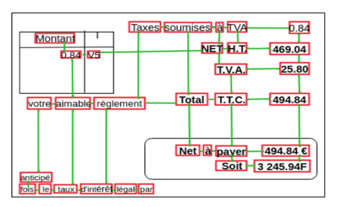
The most common way to build the graph is to represent each word on the image with a node, the rest of the information is encoded in the feature vector of each node.
Once we have created a graph representation for each of the scanned receipts, we can train a GCN to classify each node into one of the target classes (a.k.a. tags), e.g.: “company”, “address”, “date”, “total”.
Node Features
The features of a node include a representation for the word and another for the context (edges). For instance, the word can be represented as a pre trained word-embedding vector, and the context as a vector of relative distances from the current node word to other words in the image.
Most models differ in the way they construct the context representation, some model encode the distance to each other word in the image, others just encode the distance to the four closest words in each direction.
You may want to add other engineered features to achieve a richer representation, e.g.: Boolean features, like isDate, isZipCode.
Graph Creation (Feature Engineering)
There are different techniques to create this graph, most of them convert each text area into a node and they may differ on how they construct the edges. One of such techniques [2] creates a maximum of four edges for each node, the edges connect each text area to its closest four neighboring text areas in each direction (Up, Down, Left and Right).
Node Classification
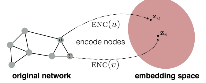
The GCN learns to embed node feature vector (combination of word embedding and the connection structure to other nodes) by generating a vector of real numbers that represents the input node as a point in an N-dimensional space, and similar nodes will be mapped to close neighboring points in the embedding space [4], allowing to train a model able to classify the nodes.
Network Architectures
The field of GCN is an active area of research and many different techniques are being proposed to compute convolutions on graphs; these can be grouped under two broad categories, as follows:
- Message Passing Neural Networks (MPNN) (a.k.a. Spatial Convolutions)
- Spectral Convolutions
Message Passing Neural Networks (MPNN)
The MPNN approach (this name may vary across the literature) is an attempt to mimic many of the advantages of vanilla convolution
Spatial convolutions scan the locality of each node, but are different than 1D or 2D convolution layers in CNNs.
The standard notion of convolution over a sequence (1D convolution) or an image (2D convolution) relies on having a regular grid, where each neighbor has well-defined neighbors, e.g. [“before” and “after”] in a sequence or ["above", "below", "to the left", "to the right"] in the case of a 2D image. On a graph structure there is usually no natural choice for an ordering of the neighbors of a node (Fout et al., 2017, Protein Interface Prediction using Graph Convolutional Networks). This has motivated models that represent the dependency on neighboring nodes (the filter) as a bag of weights (a set), to learn an order-independent function, as the following:

where Ni is the set of neighbors of node i, WC is the weight matrix associated with the center node, WN is the weight matrix associated with neighboring nodes, and b is a vector of biases, one for each filter. The dimensionality of the weight matrices is determined by the dimensionality of the inputs and the number of filters.
(Fout et al., 2017, Protein Interface Prediction using Graph Convolutional Networks)
Observe that the same matrix of weights WC applies to all of the neighbors, therefore there is no assumption of order or relative position in this model (the order in which you visit the neighbours does not affect the result) and only the features of each node matter.
Inference
Once the model has been trained, the weight matrices can be applied to any graph of unseen structure, because the weights are independent of the number of neighbours of each node, and therefore independent of the connection structure of the graph.
Applied to the multiple-graph use case, this architecture naturally supports inference on a single example.
Spectral Convolutions
Spectral methods work by transforming the input features to the spectral domain, this means decomposing the input into a combination (usually, a sum) of simple elements. which are orthogonal, and therefore form a basis.
Spectral graph convolutions do not scan the input feature matrix sliding a filter (like a regular 1D or 2D convolution layers, instead they exploit the Convolution Theorem from signal processing, which states that an expensive convolution in the spatial domain can be computed as a cheap multiplication by transforming the signals first to the frequency domain. In other words, the Fourier transform of a convolution of two functions is the element-wise product of their Fourier transforms. Applying the convolution theorem reduces the computational complexity of the convolution from O(n2) to O(n log n).
In signal processing, the Discrete Fourier Transform is used to transform a signal to the frequency domain, this consists of the matrix multiplication of a signal with a special basis, known as the DFT matrix (Spectral Graph Convolution Explained and Implemented Step By Step).
The DFT basis assumes a regular grid, which is not the typical case on graphs. For that reason, a more general (and computationally expensive) basis must be used, which is eigenvectors V of the graph Laplacian L. Fortunately, the Convolution Theorem also applies to the Laplacian transform, but the eigenvectors must be found by eigen-decomposition: L=VΛVᵀ, where Λ are eigenvalues of L, which is a computationally expensive operation, so a simplified approximation is needed.
Inference
Inference with a Spectral GCN is slightly peculiar, since the model only works on a network with a fixed number of nodes. The idea is to use a semi-supervised learning setting. The model takes as input a partially-labeled dataset and outputs labels for all the nodes (including those that where unlabeled in the input).
This applicability of this kind of GCN to the multiple-graph use case is discussed later in this same article.
Approximate Convolutions on Graphs
The author of this paper (Kipf, 2017), proposes to the following forward-propagation formula to model a spectral convolutional layer:
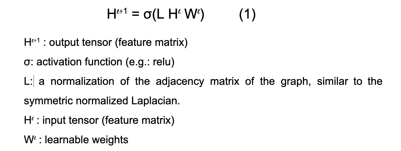
Note that L is not a learnable parameter, and is the same for all layers. In Kipf’s approximate convolutions on graphs, L is precomputed according to this formula:

Replacing L in the above by its components:

The above formula is motivated from Spectral Graph Convolutions, a concept from the field of Signal Processing (Hammond, 2011).
Spectral Convolutions Applied to Receipts IE
One of the advantages of spectral convolutions is that they can be computed using fast approximations.
The main weakness of Spectral Convolution methods is that they are only useful for learning patterns on the graph that they were trained for.
This tends to fit those datasets that consist of a single large network, like a social network, or a literary reference network, but it does not model correctly those datasets where each input example is potentially a different graph. In the case of a dataset of invoices, each document can have a different layout, resulting in a different graph adjacency matrix and a different set of calculated eigenvalues, the weights learned with the eigenvalues from one invoice do not apply to the next.
So the challenge for anyone trying to use spectral convolutinos on invoice datasets is to create a network architecture that learn different sets of weights for all the different types of eigenvalues found in the training set, and hope that this model will have learn patterns that are generalizable enough to the test invoices with unseen graph connection structure.
In [4] this challenge is met by network architecture that stacks up 4 GCN layers, the first layer learns 16 different filters, note that this can learn 16 different graph connection patterns, and the second layer learn 32 filters, learning to recognize 32 combinations of the 16 patterns learned in layer 1. This hierarchical compositionality property, also found in CNN’s, gives the model the power to generalize to unseen layouts.
Code Overview
The Information Extraction pipeline consists of the following steps:
- Graph Modeler (create a graph from the ‘words’ files)
- Feature Calculator (save features, adj. matrix)
- Data Loader (load features, adj. matrix and labels in memory)
- GCN Semi-Supervised Learning Process (Training and Prediction)
The ‘words’ files - each one contains the words (one string per line) extracted from one image with an OCR software.
The second set is the text files that contain the tags (aka labels), manually created by annotators.
The output of the pipeline, is the predicted label (tag) for each one of the words in the test set.
Images and Annotations
Due to the sensitive information contained in invoices, it is very rare to find a publicly available dataset of invoices, so we are going to use a dataset of Receipts provided by end users.
The dataset contains three types of files
- Images: 1000 whole scanned receipt images.
- Labels file: one text file for each image, containing the items items extracted via OCR.: Each receipt image has been processed by an OCR engine, which extracted dozens of words from each image, consisting mainly of digits and English characters. Each word is stored as a separate row, preceded by the coordinates of its location on the image.
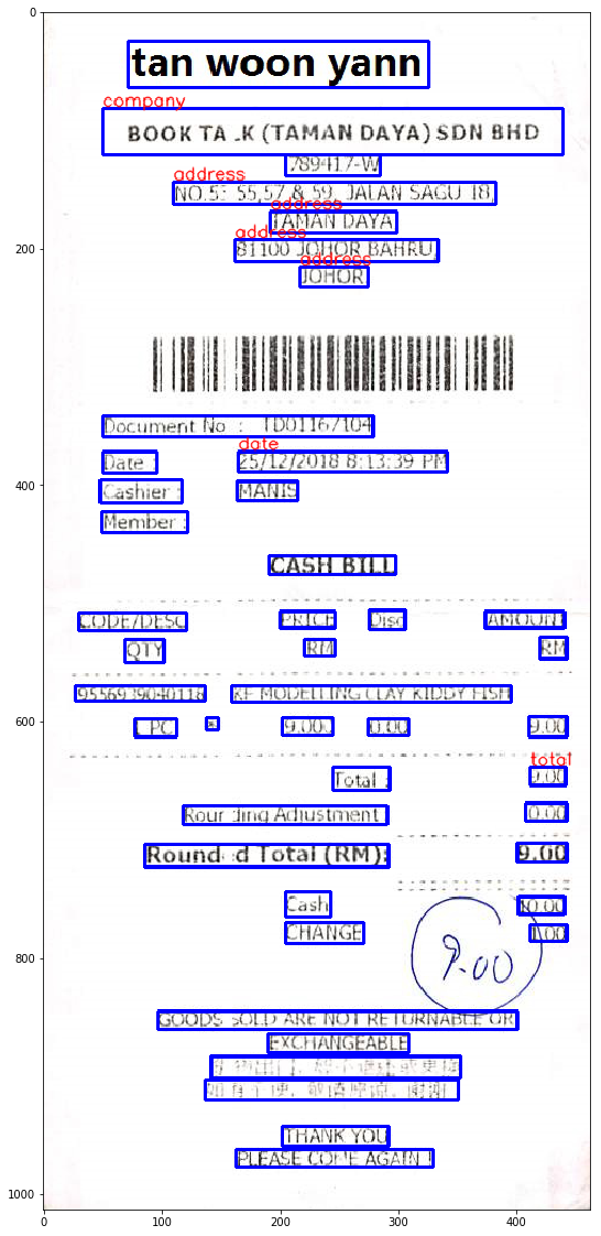
- Tags: Additionally, each image has been manually annotated, tagging four key fields, such as company name, date, address and total cost. The tags are stored as key-value pairs in a JSON file.
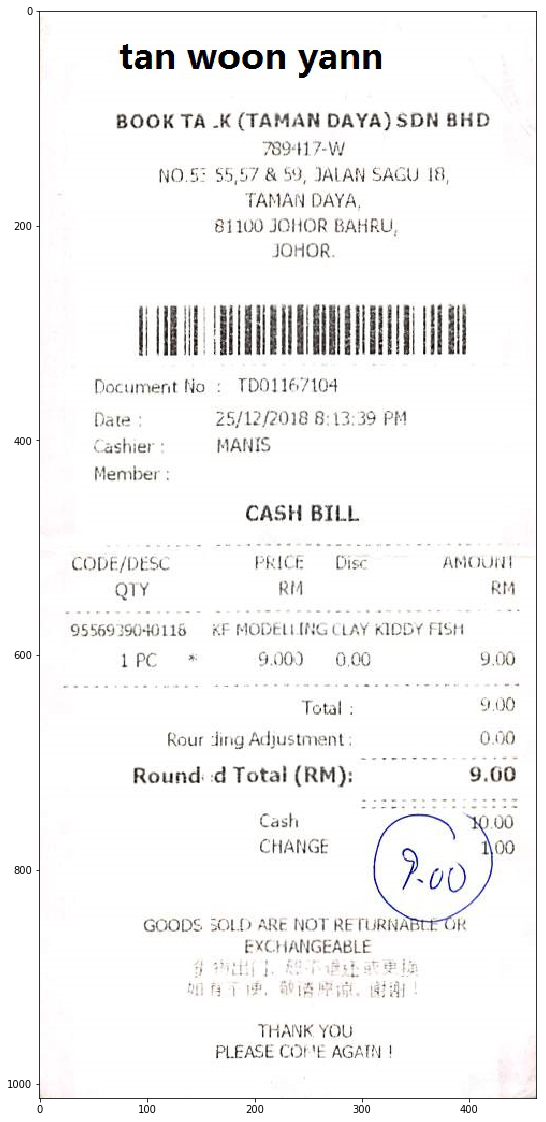
The following picture shows the image with the labels in blue and the tags written on top of the tagged field (red font).
Graph Modeler
The Graph Modeler module finds the nearest neighbors in the four main directions (Left, Top, Right, Bottom) for each word in the image.
The input is a list of text lines each element is a line that represents a word extracted from the image, these lines are sorted by vertical position from top to bottom.
The output is a graph, stored in a python dictionary, where each (key, value) pair corresponds to a node in the graph and represents a word (a text line in the input list).
The key is an index to the word Area tuple in the word_areas list, and the value is a dictionary of edges, where each (key, value) pair is an edge to a nearest neighbour, the key is the direction ('left', 'right', 'top', 'bottom') and the value is a tuple (index_to_word, relative_distance), for example: ('left': (5, 0.1)) represents an edge to the left neighbor word (5 is an index in a list where all the words are loaded.)
# ------------------------------------------------------------------------
### Runs graph modeling process
# ------------------------------------------------------------------------
def run_graph_modeler(normalized_dir, target_dir):
    print("Running graph modeler")

    img_files, word_files, _ = \
    get_normalized_filepaths(normalized_dir)

    for img_file, word_file in zip(img_files, word_files):
        # reads normalized data for one image
        img, word_areas, _ = load_normalized_example(img_file, word_file)

        # computes graph adj matrix for one image
        lines = line_formation(word_areas)
        width, height = cv_size(img)
        graph = graph_modeling(lines, word_areas, width, height)
        adj_matrix = form_adjacency_matrix(graph)

        # saves node features and graph
        save_graph(target_dir, img_file, graph, adj_matrix)
The main loop of the graph modeler process
Feature Calculator
The Feature Calculator computed features for every node, there are three types of features: word embeddings (computed used pretrained embeddings), neighbor relative distances (extracted from the graph), and binary features (eg.: numeric, alphabetic, etc.)
The feature calculator reads the words and calls the Graph Modeler to create a graph, then extracts some features from the graph.
# -------------------------------------------------------------------------
#### Numeric Features (neighbour distances from graph)
# -------------------------------------------------------------------------
def get_word_area_numeric_features(word_area, graph):
    """
    Extracts numeric features from the graph: returns 4 floats
    between -1 and 1 that represent the the relative distance
    to the nearest neighbour in each of the four main directions.
    Fills the "undefined" values with the null distance (0)
    """
    edges = graph[word_area.idx]
    get_numeric = lambda x: x if x != UNDEFINED else 0
    rd_left   = get_numeric(edges["left"][1])
    rd_right  = get_numeric(edges["top"][1])
    rd_top    = get_numeric(edges["right"][1])
    rd_bottom = get_numeric(edges["bottom"][1])
    return [rd_left, rd_right, rd_top, rd_bottom]
Numeric Features extracted from the graph (only the 4 edges per node, as explained in the Graph Modeler section)
The Feature Calculator also extracts features directly from the words, in this case, sub-word embeddings are used as a way to avoid out-of-dictionary words.
Finally, the Feature Extractor forms a feature vector of size 318 (an array of floats) for each word and stores it as a .csv in the features folder (one file for each image).
Data Loader
The main purpose of the data loader is to compose a batch graph, this is a single graph that contains all the individual graphs of all the images. Some of the images graphs (training set) have labels for some of their nodes (tags for some of the words), other image graphs do not have labels. The batch graph is composed by joining all the individual image graphs adjacency matrices into a block-diagonal sparse matrix. The individual image graphs remain non-linked between themselves.
The main purpose of the data_loader is to convert a batch of individual graphs into a single large graph of non-linked graphs.
Model Runner
The Model Runner module runs the semi-supervised learning process. The semi-supervised setting allows the model to perform transductive learning, exploiting the relations between neighbouring feature vectors.
The original code GCN class has been extended to support a variable number of layers (see class GCNX in the gcn/models.py file):
for i in range(1, FLAGS.num_hidden_layers):
        in_dim = FLAGS.hidden1 * 2**(i-1)
        out_dim = in_dim * 2
        self.layers.append(GraphConvolution(input_dim=in_dim,
                                            output_dim=out_dim,
                                            placeholders=self.placeholders,
                                            act=tf.nn.relu,
                                            dropout=True,
                                            logging=self.logging))
GCN Layer
At the core of the modeling code, in the gcn/layers.py file, is the GraphConvolution class which defines the GCN layer as a modified fully-connected (a.k.a. Dense or Linear) layer.
The GCN layer is a Dense layer modified with multiple sets of weights and extra matrix multiplications that, in theory, transform the features to the spectral domain and back; the spectral transform is simplified by a linear approximation using the Chebyshev coefficients, the best way to appreciate this is comparing the forward transform in GCN, vs. the Dense layer.
# transform
output = dot(x, self.vars['weights'])
Regular Dense Layer forward transform (simplified for clarity)
# convolve
supports = list()
for i in range(len(self.support)):
pre_sup = dot(x, self.vars['weights_' + str(i)])
support = dot(self.support[i], pre_sup, sparse=True)
supports.append(support)
output = tf.add_n(supports)
GCN Layer forward transform (simplified for clarity)
Each layer has k sets of weights, where k = len(self.support). Each element in the list self.support contains a matrix of Chebyshev coefficients that represent an additional hop of propagation over the graph connectivity structure, that is: self.support[0] computes interactions between words that are 1 edge apart (neighbors), self.support[1] computes interactions between words that are 2 edges apart (neighbors of neighbors), etc. The GraphConvolution layer learns a set of weights for each support level (the self.support list contains k levels). Finally, all the weighted support levels are added to produce the approximated graph convolution.
The parameters for the runner are imported as constants from a common python script.
# global parameters

from collections import namedtuple

# named tuples
WordArea = namedtuple('WordArea', 'left, top, right, bottom, content, idx')
TrainingParameters = namedtuple("TrainingParameters", "dataset model learning_rate epochs hidden1 num_hidden_layers dropout weight_decay early_stopping max_degree data_split")

# trainig parameters:
# --------------------------------------------------------------------------------
# dataset:        Selectes the dataset to run on
# model:          Defines the type of layer to be applied
# learning_rate:  Initial learning rate.
# epochs:         Number of epochs to train.
# hidden1:        Number of units in hidden layer 1.
# dropout:        Dropout rate (1 - keep probability).
# weight_decay:   Weight for L2 loss on embedding matrix.
# early_stopping: Tolerance for early stopping (# of epochs).
# max_degree:     Maximum Chebyshev polynomial degree.
FLAGS = TrainingParameters('receipts', 'gcnx_cheby', 0.001, 200, 16, 2, 0.6, 5e-4, 10, 3, [.4, .2, .4])

# output classes
UNDEFINED="undefined"
CLASSES = ["company", "date", "address", "total", UNDEFINED]
Global parameters controlling the execution.
During data preprocessing, a function is called to calculate the Chebyshev approximation coefficients, these are computed from the adj matrix.
if FLAGS.model == 'gcnx_cheby':
    support = chebyshev_polynomials(adj, FLAGS.max_degree)
    num_supports = 1 + FLAGS.max_degree
    model_func = GCNX
References
- An Overview of the Tesseract OCR Engine (Ray Smith, Google, 2007)
- [1906.01969] Efficient, Lexicon-Free OCR using Deep Learning
- [1906.07155] MMDetection: Open MMLab Detection Toolbox and Benchmark
- An Invoice Reading System Using a Graph Convolutional Network
- Overview - ICDAR 2019 Robust Reading Challenge on Scanned Receipts OCR and Information Extraction - ICDAR 2019
- [1609.02907] Semi-Supervised Classification with Graph Convolutional Networks
Further Reading
- Graph Convolution for Multimodal Information Extraction from Visually Rich Documents
- Cardinal Graph Convolution Framework for Document Information Extraction
- Convolutional Neural Networks for Direct
Text Deblurring
Update:
Added further reading material around using Graph Convolutional Neural Network for extracting information from documents like receipts using receipt OCR.