A 2019 guide to Human Pose Estimation with Deep Learning

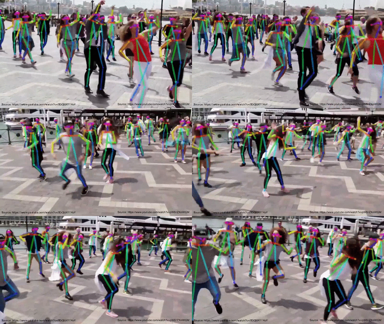
Human Pose estimation is an important problem that has enjoyed the attention of the Computer Vision community for the past few decades. It is a crucial step towards understanding people in images and videos. In this post, I write about the basics of Human Pose Estimation (2D) and review the literature on this topic. This post will also serve as a tutorial in Human Pose Estimation and can help you learn the basics.

What is Human Pose Estimation?

Human Pose Estimation is defined as the problem of localization of human joints (also known as keypoints - elbows, wrists, etc) in images or videos. It is also defined as the search for a specific pose in space of all articulated poses.

2D Pose Estimation - Estimate a 2D pose (x,y) coordinates for each joint from a RGB image.
3D Pose Estimation - Estimate a 3D pose (x,y,z) coordinates a RGB image.

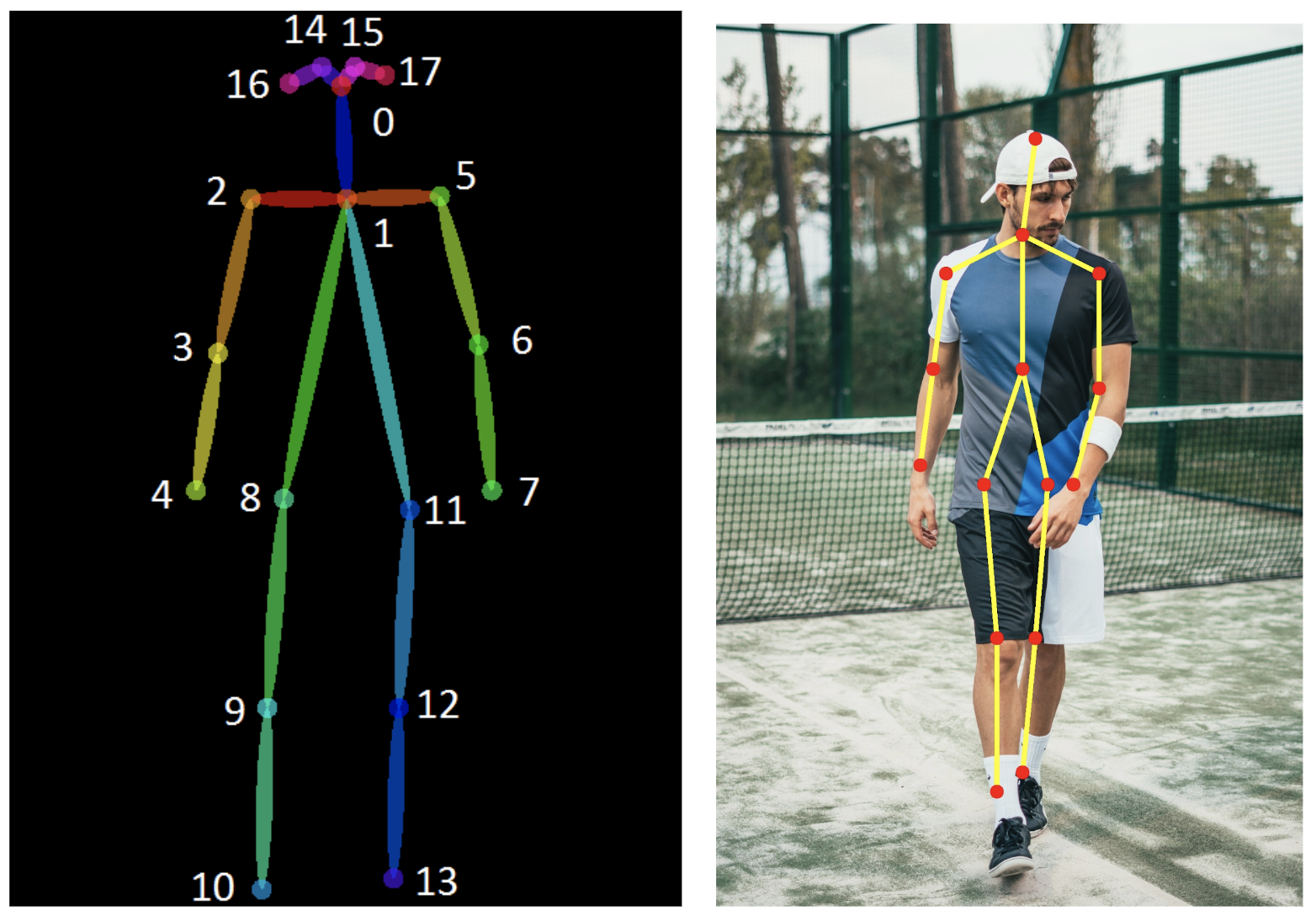
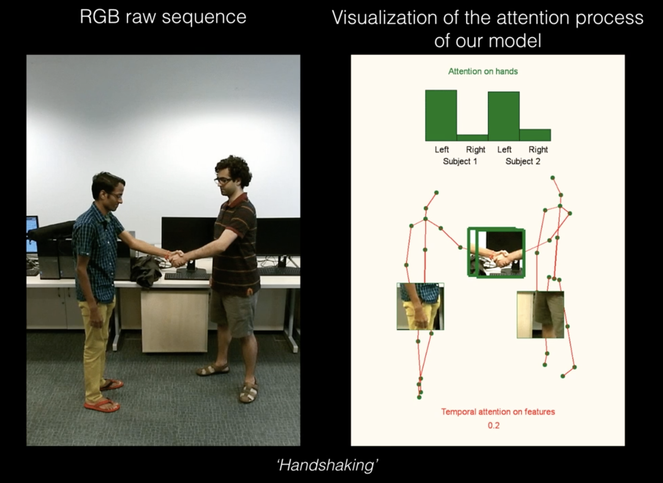
Human Pose Estimation has some pretty cool applications and is heavily used in Action recognition, Animation, Gaming, etc. For example, a very popular Deep Learning app HomeCourt uses Pose Estimation to analyse Basketball player movements.

Why is it hard?

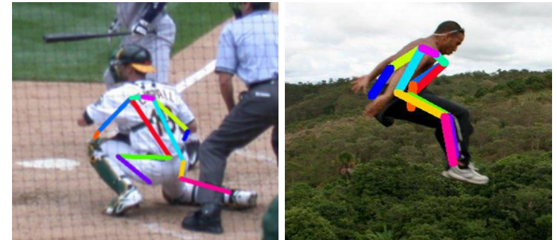
Strong articulations, small and barely visible joints, occlusions, clothing, and lighting changes make this a difficult problem.

I will be covering 2D human pose estimation in this post and 3D pose estimation in the next one.

Different approaches to 2D Human Pose Estimation

Classical approaches

• The classical approach to articulated pose estimation is using the pictorial structures framework. The basic idea here is to represent an object by a collection of "parts" arranged in a deformable configuration (not rigid). A "part" is an appearance template which is matched in an image. Springs show the spatial connections between parts. When parts are parameterized by pixel location and orientation, the resulting structure can model articulation which is very relevant in pose estimation. (A structured prediction task)

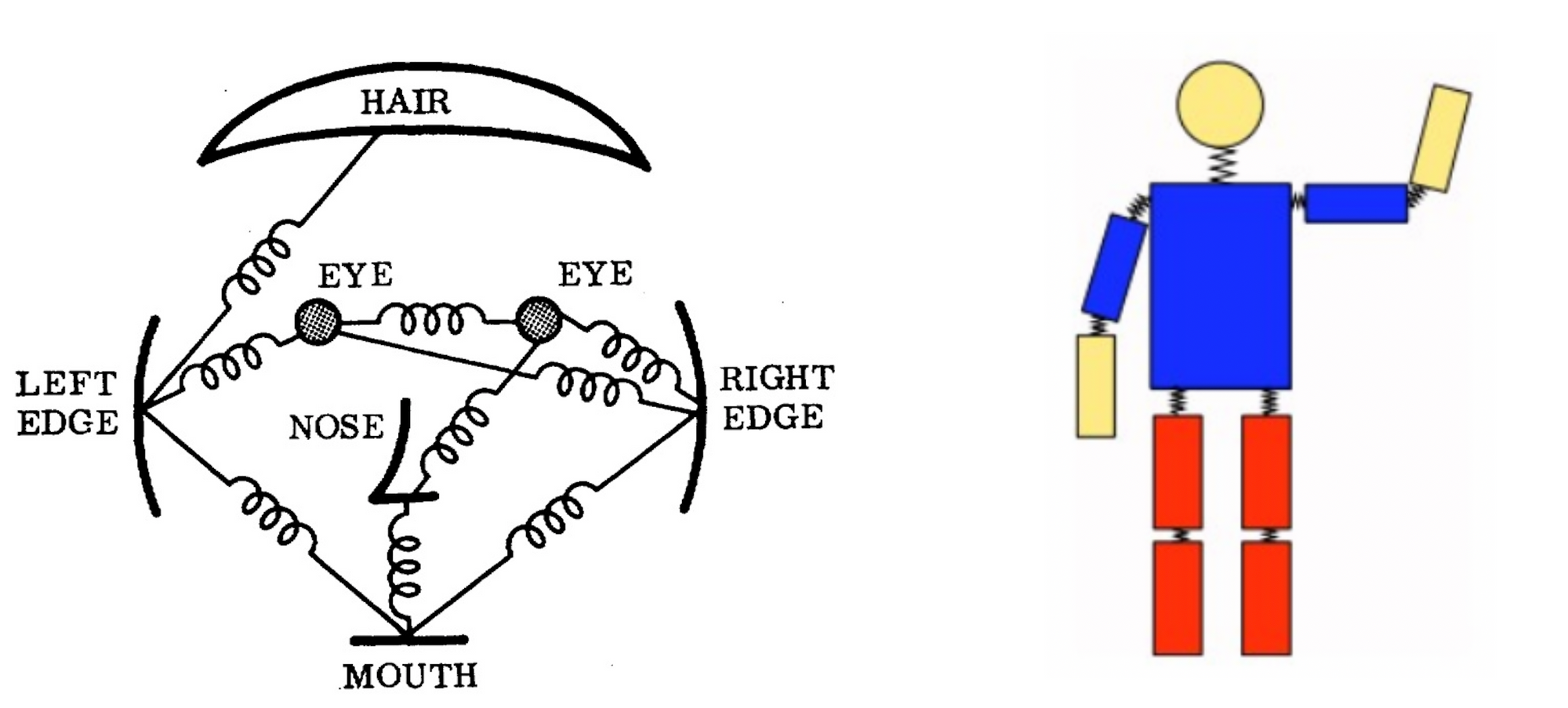
• The above method, however, comes with the limitation of having a pose model not depending on image data. As a result, research has focused on enriching the representational power of the models.
• Deformable part models - Yang and Ramanan use a mixture model of parts which expresses complex joint relationships. Deformable part models are a collection of templates arranged in a deformable configuration and each model has global template + part templates. These templates are matched for in an image to recognize/detect an object. The Part-based model can model articulations well. This is however achieved at the cost of limited expressiveness and does not take in global context into account.

Deep Learning based approaches

The classical pipeline has its limitations and Pose estimation has been greatly reshaped by CNNs. With the introduction of “DeepPose” by Toshev et al, research on human pose estimation began to shift from classic approaches to Deep Learning. Most of the recent pose estimation systems have universally adopted ConvNets as their main building block, largely replacing hand-crafted features and graphical models; this strategy has yielded drastic improvements on standard benchmarks.

In the next section, I’ll summarize a few papers in chronological order that represents the evolution of Human Pose Estimation starting with DeepPose from Google (This is not an exhaustive list, but a list of papers that I feel show the best progression/most significant ones per conference).

Papers covered

1.    DeepPose

2.    Efficient Object Localization Using Convolutional Networks

3.    Convolutional Pose Machines

4.    Human Pose Estimation with Iterative Error Feedback

5.    Stacked Hourglass Networks for Human Pose Estimation

6.   Simple Baselines for Human Pose Estimation and Tracking

7.    Deep High-Resolution Representation Learning for Human Pose Estimation

DeepPose: Human Pose Estimation via Deep Neural Networks (CVPR’14) [arXiv]

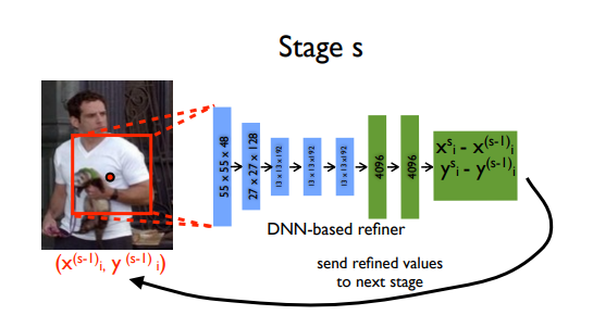
DeepPose was the first major paper that applied Deep Learning to Human pose estimation. It achieved SOTA performance and beat existing models. In this approach, pose estimation is formulated as a CNN-based regression problem towards body joints. They also use a cascade of such regressors to refine the pose estimates and get better estimates. One important thing this approach does is the reason about pose in a holistic fashion, i.e even if certain joints are hidden, they can be estimated if the pose is reasoned about holistically. The paper argues that CNNs naturally provide this sort of reasoning and demonstrate strong results.

Model

The model consisted of an AlexNet backend (7 layers) with an extra final layer that outputs 2k joint coordinates - \(\left(x_{i}, y_{i}\right) * 2\) for \(i \in\{1,2 \ldots k\}\) (where \(k\) is the number of joints).

The model is trained using a \(L2\) loss for regression.

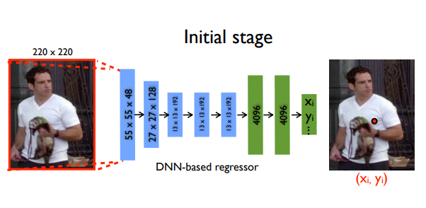
An interesting idea this model implements is refinement of the predictions using cascaded regressors. Initial coarse pose is refined and a better estimate is achieved. Images are cropped around the predicted joint and fed to the next stage, in this way the subsequent pose regressors see higher resolution images and thus learn features for finer scales which ultimately leads to higher precision.

Results

PCP is used on LSP (Leeds sports dataset) and FLIC (Frames Labeled In Cinema). Have a look at the appendix to find the definitions of some of the popular evaluation metrics like PCP & PCK.

Comments

• This paper applied Deep Learning (CNN) to Human Pose Estimation and pretty much kicked off research in this direction.
• Regressing to XY locations is difficult and adds learning complexity which weakens generalization and hence performs poorly in certain regions.

• Recent SOTA methods transform the problem to estimating \(K\) heatmaps of size \(W_0 × H_0 , \{H_1, H_2, . . . , H_k\}\), where each heatmap \(H_k\) indicates the location confidence of the \(k\)th keypoint. (K keypoints in total). The next paper was fundamental in introducing this idea.

Efficient Object Localization Using Convolutional Networks (CVPR’15) [arXiv]

This approach generates heatmaps by running an image through multiple resolution banks in parallel to simultaneously capture features at a variety of scales. The output is a discrete heatmap instead of continuous regression. A heatmap predicts the probability of the joint occurring at each pixel. This output model is very successful and a lot of the papers that followed predict heatmaps instead of direct regression.

Model

A multi-resolution CNN architecture (coarse heatmap model) is used to implement a sliding window detector to produce a coarse heatmap output.

The main motivation of this paper is to recover the spatial accuracy lost due to pooling in the initial model. They do this by using an additional ‘pose refinement’ ConvNet that refines the localization result of the coarse heat-map. However, unlike a standard cascade of models, they reuse existing convolution features. This not only reduces the number of trainable parameters in the cascade but also acts as a regulariser for the coarse heat-map model since the coarse and fine models are trained jointly.

In essence, the model consists of the heat-map-based parts model for coarse localization, a module to sample and crop the convolution features at a specified \((x, y)\) location for each joint, as well as an additional convolutional model for fine-tuning.

A critical feature of this method is the joint use of a ConvNet and a graphical model. The graphical model learns typical spatial relationships between joints.

Training

The model is trained by minimizing the Mean Squared-Error (MSE) distance of our predicted heat-map to a target heat-map (The target is a 2D Gaussian of constant variance (σ ≈ 1.5 pixels) centered at the ground-truth \((x, y)\) joint location)

Results

Comments

• Heatmaps work better than direct joint regression
• Joint use of a CNN and Graphical Model

• However, these methods lack structure modelling. The space of 2D human poses is highly structured because of body part proportions, left-right symmetries, interpenetration constraints, joint limits (e.g. elbows do not bend back) and physical connectivity (e.g. wrists are rigidly related to elbows), among others. Modelling this structure should make it easier to pinpoint the visible keypoints and make it possible to estimate the occluded ones. The next few papers tackle this, in their own novel ways.

Convolutional Pose Machines (CVPR’16) [arXiv] [code]

Summary

• This is an interesting paper that uses something called a Pose machine. A pose machine consists of an image feature computation module followed by a prediction module. Convolutional Pose Machines are completely differentiable and their multi-stage architecture can be trained end to end. They provide a sequential prediction framework for learning rich implicit spatial models and work very well for Human pose.
• One of the main motivations of this paper is to learn long range spatial relationships and they show that this can be achieved by using larger receptive fields.

Model

g1() and g2() predict heatmaps (belief maps in the paper). Above is a high level view. Stage 1 is the image feature computation module, and Stage 2 is the prediction module. Below is a detailed architecture. Notice how the receptive fields increase in size?

A CPM can consist of > 2 Stages, and the number of stages is a hyperparameter. (Usually = 3). Stage 1 is fixed and stages > 2 are just repetitions of Stage 2. Stage 2 take heatmaps and image evidence as input. The input heatmaps add spatial context for the next stage. (Has been discussed in detail in the paper).

On a high level, the CPM refines the heatmaps through subsequent stages.

The paper used intermediate supervision after each stage to avoid the problem of vanishing gradients, which is a common problem for deep multi-stage networks

Results

• MPII:  PCKh-0.5 score achieves state of the art at 87.95%, which is 6.11% higher than the closest competitor, and it is noteworthy that on the ankle (the most challenging part), our PCKh@0.5 score is 78.28% which is 10.76% higher than the closest competitor.
• LSP: Model achieves state of the art at 84.32% (90.5% when adding MPII training data).

Comments

• Introduced a novel CPM framework that showed SOTA performance of MPII, FLIC and LSP datasets.

Human Pose Estimation with Iterative Error Feedback (CVPR’16) [arXiv] [code]

Summary

This is a pretty dense paper and I’ve tried to summarize it briefly without leaving out too much. The overall working is pretty straightforward: Predict what is wrong with the current estimates and correct them iteratively. To quote the authors, Instead of directly predicting the outputs in one go, they use a self-correcting model that progressively changes an initial solution by feeding back error predictions, and this process is called Iterative Error Feedback (IEF).

Let’s jump right to the model pipeline.

• The input consists of the image I and a representation of the previous output \(y_{t-1}\). Keep in mind this is an iterative process and the same output is refined over steps.
• Input, \(x_{t}=I \oplus g\left(y_{t-1}\right)\) where \(I\) is the image and \(y_{t-1}\) is the previous output
  • \(f\left(x_{t}\right)\) outputs the correction \(\varepsilon_{t}\) and this added to the current output \(y_{t}\) to generate \(y_{t+1},\) which takes the corrections into account.
  • \(g\left(y_{t+1}\right)\) converts each keypoint in \(y_{t+1}\) into a heatmap channel so they can be stacked to the image \(I,\) so as to form the input for the next teration. This process is repeated \(T\) times till we get a refined \(y_{t+1}\) and is brought closer to the ground truth by the addition of \(\varepsilon_{t}\)

• Mathematically,

  • \(\epsilon_{t}=f\left(x_{t}\right)\)
  • \(y_{t+1}=y_{t}+\epsilon_{t}\)
  • \(x_{t+1}=I \oplus g\left(y_{t+1}\right)\)

• \(f()\) and \(g()\) are learnable and \(f()\) is a CNN

• One important point to note is that as the ConvNet \(f()\) takes \(I \oplus g\left(y_{t}\right)\) as inputs, it has the ability to learn features over the joint input-output space, which is pretty cool.

• The parameters \(\Theta_{g}\) and \(\Theta_{f}\) are learnt by optimizing the below equation:

  • \(\min_{\Theta_{f},\Theta_{g}}\sum_{t=1}^{T}h\left(\epsilon_{t},e\left(y, y_{t}\right)\right)\)
  • where, \(\varepsilon_{t}\) and \(e\left(y, y_{t}\right)\) are predicted, and target corrections respectively. The function \(h\) is a measure of distance, such as a quadratic loss. \(T\) is the number of correction steps taken by the model.

Example

As you can see, the pose is refined over the correction steps.

Results

Comments

An elegant paper that introduces a good novelty and works very well.

Stacked Hourglass Networks for Human Pose Estimation (ECCV’16) [arXiv] [code]

This is a landmark paper that introduced a novel and intuitive architecture and beat all previous methods. It’s called a stacked hourglass network since the network consists of steps of pooling and upsampling layers which looks like an hourglass, and these are stacked together. The design of the hourglass is motivated by the need to capture information at every scale. While local evidence is essential for identifying features like faces hands, a final pose estimate requires global context. The person’s orientation, the arrangement of their limbs, and the relationships of adjacent joints are among the many cues that are best recognized at different scales in the image (Smaller resolutions capture higher order features and global context).

The network performs repeated bottom-up, top-down processing with intermediate supervision
- Bottom-up processing (from high resolutions to low resolutions)
- Top-down processing (from low resolutions to high resolutions)

The network uses skip connections to preserve spatial information at each resolution and passes it along for upsampling, further down the hourglass.

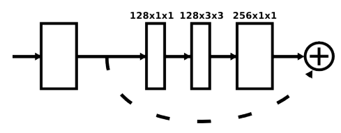
Each box is a  residual module like the below figure;

Intermediate supervision

Intermediate supervision is applied to the predictions of each hourglass stage, i.e the predictions of each hourglass in the stack are supervised, and not only the final hourglass predictions.

Results

Why does it work so well?

The hourglass captures information at every scale. This way, global and local information and captured completely and are used by the network to learn the predictions.

Simple Baselines for Human Pose Estimation and Tracking (ECCV’18) [paper] [code]

The previous approaches work very well but are complex. This work follows the question – how good could a simple method be? And achieved the state-of-the-art at mAP of 73.7% on COCO.

The network structure is quite simple and consists of a ResNet + few deconvolutional layers at the end. (Probably the simplest way to estimate heat maps)

While the hourglass network uses upsampling to increase the feature map resolution and puts convolutional parameters in other blocks, this method combines them as deconvolutional layers in a very simple way. It was quite surprising to see such a simple architecture perform better than one with skip connections that preserve the information for each resolution.

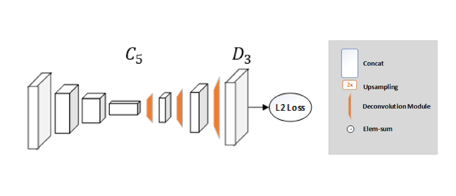
Mean Squared Error (MSE) is used as the loss between the predicted heatmaps and targeted heatmaps. The targeted heatmap \(H^{k}\) for joint \(k\) is generated by applying a 2D Gaussian centered on the kth joint’s ground truth location with std dev = 1 pixel.

Results

Deep High-Resolution Representation Learning for Human Pose Estimation [HRNet] (CVPR’19) [arXiv] [code]

The HRNet (High-Resolution Network) model has outperformed all existing methods on Keypoint Detection, Multi-Person Pose Estimation and Pose Estimation tasks in the COCO dataset and is the most recent. HRNet follows a very simple idea. Most of the previous papers went from a high → low → high-resolution representation. HRNet maintains a high-resolution representation throughout the whole process and this works very well.

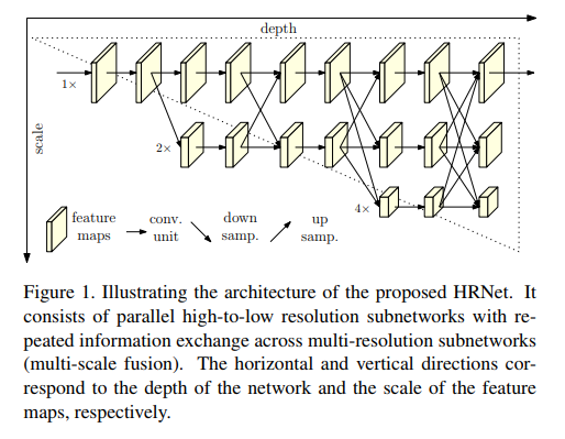
The architecture starts from a high-resolution subnetwork as the first stage, and gradually adds high-to-low resolution subnetworks one by one to form more stages and connect the multi-resolution subnetworks in parallel.

Repeated multi-scale fusions are conducted by exchanging information across parallel multi-resolution subnetworks over and over through the whole process.

Another pro is that this architecture does not use intermediate heatmap supervision, unlike the Stacked Hourglass.

Heatmaps are regressed using an MSE loss, similar to simple baselines. (add in article link)

Results

Here are a few other papers that I feel are interesting:

• Flowing ConvNets for Human Pose Estimation in Videos (ICCV’15) [arXiv]
• Learning Feature Pyramids for Human Pose Estimation (ICCV’17)  [arXiv]  [code]
• Realtime Multi-Person 2D Pose Estimation using Part Affinity Fields (CVPR’17) [arXiv] [code]: Very popular real-time multi-person pose estimator (Better known as OpenPose)

• Multi-Context Attention for Human Pose Estimation (CVPR’17) [arXiv] [code]
• Cascaded Pyramid Network for Multi-Person Pose Estimation (CVPR’18) [arXiv] [code]

Appendix

Common Evaluation Metrics

Evaluation metrics are needed to measure the performance of human pose estimation models.

Percentage of Correct Parts - PCP: A limb is considered detected  (a correct part) if the distance between the two predicted joint locations and the true limb joint locations is less than half of the limb length (Commonly denoted as PCP@0.5).

• It measures the detection rate of limbs. The con is that it penalizes shorter limbs more since shorter limbs have smaller thresholds.
• Higher the PCP, better the model.

Percentage of Correct Key-points - PCK: A detected joint is considered correct if the distance between the predicted and the true joint is within a certain threshold. The threshold can either be:

• PCKh@0.5 is when the threshold = 50% of the head bone link
• PCK@0.2 == Distance between predicted and true joint < 0.2 * torso diameter
• Sometimes 150 mm is taken as the threshold.
• Alleviates the shorter limb problem since shorter limbs have smaller torsos and head bone links.
• PCK is used for 2D and 3D (PCK3D). Again, the higher the better.

Percentage of Detected Joints - PDJ: A detected joint is considered correct if the distance between the predicted and the true joint is within a certain fraction of the torso diameter. PDJ@0.2 = distance between predicted and true joint < 0.2 * torso diameter.

Object Keypoint Similarity (OKS) based mAP:

• Commonly used in the COCO keypoints challenge.
• OKS =

$$
\frac{\sum_{i} \exp \left(-d_{i}^{2} / 2 s^{2} k_{i}^{2}\right) \delta\left(v_{i}>0\right)}{\sum_{i} \delta\left(v_{i}>0\right)}
$$

• Where \(d_{i}\) is the Euclidean distance between the detected keypoint and the corresponding ground truth, \(v_{i}\) is the visibility flag of the ground truth, s is the object scale, and \(k_{i}\)s a per-keypoint constant that controls falloff.

• To put it simply, OKS plays the same role that IoU plays in object detection. It is calculated from the distance between predicted points and ground truth points normalized by the scale of the person. More info Typically, standard average precision and recall scores are reported in papers: \(A P^{50}\) (AP at OKS = 0.50) \(A P^{75}\) , \(A P\) (the mean of \(A P\) scores at 10 positions, OKS = 0.50, 0.55, . . . , 0.90, 0.95; \(A P^{M}\) for medium objects, \(A P^{L}\) for large objects, and \(A R\) (Average recall) at OKS = 0.50, 0.55, . . . , 0.90, 0.955.

Lazy to code, don't want to spend on GPUs? Head over to Nanonets and build computer vision models for free!